Loading data into machine learning¶

In this notebook, we will look at the necessary steps required before any machine learning takes place.

load the data
look at the variables in the dataset, in particular, differentiate between numerical and categorical variables, which need different preprocessing in most machine learning workflows
visualize the distribution of the variables to gain some insights into the dataset

Loading the adult census dataset¶

We will use data from the “Current Population adult_census” from 1994 that we downloaded from OpenML.

import pandas as pd

adult_census = pd.read_csv("../datasets/adult-census.csv")

We can look at the OpenML webpage to learn more about this dataset: http://www.openml.org/d/1590

The goal with this data is to predict whether a person earns over 50K a year from heterogeneous data such as age, employment, education, family information, etc.

The variables (columns) in the dataset¶

The data are stored in a pandas dataframe.

Pandas is a Python library to manipulate tables, a bit like Excel but programming: https://pandas.pydata.org/

adult_census.head()  # Look at the first few lines of our dataframe

	age	workclass	fnlwgt	education	education-num	marital-status	occupation	relationship	race	sex	capital-gain	hours-per-week	native-country	class
0	25	Private	226802	11th	7	Never-married	Machine-op-inspct	Own-child	Black	Male	0	40	United-States	<=50K
1	38	Private	89814	HS-grad	9	Married-civ-spouse	Farming-fishing	Husband	White	Male	0	50	United-States	<=50K
2	28	Local-gov	336951	Assoc-acdm	12	Married-civ-spouse	Protective-serv	Husband	White	Male	0	40	United-States	>50K
3	44	Private	160323	Some-college	10	Married-civ-spouse	Machine-op-inspct	Husband	Black	Male	7688	40	United-States	>50K
4	18	?	103497	Some-college	10	Never-married	?	Own-child	White	Female	0	30	United-States	<=50K

The column named class is our target variable (i.e., the variable which we want to predict). The two possible classes are <= 50K (low-revenue) and > 50K (high-revenue). The resulting prediction problem is therefore a binary classification problem, while we will use the other columns as input variables for our model.

target_column = 'class'
adult_census[target_column].value_counts()

 <=50K    37155
 >50K     11687
Name: class, dtype: int64

Note: classes are slightly imbalanced. Class imbalance happens often in practice and may need special techniques for machine learning. For example in a medical setting, if we are trying to predict whether patients will develop a rare disease, there will be a lot more healthy patients than ill patients in the dataset.

The dataset contains both numerical and categorical data. Numerical values can take continuous values for example age. Categorical values can have a finite number of values, for example native-country.

numerical_columns = [
    'age', 'education-num', 'capital-gain', 'capital-loss',
    'hours-per-week']
categorical_columns = [
    'workclass', 'education', 'marital-status', 'occupation',
    'relationship', 'race', 'sex', 'native-country']
all_columns = numerical_columns + categorical_columns + [
    target_column]

adult_census = adult_census[all_columns]

Note that for simplicity, we have ignored the “fnlwgt” (final weight) column that was crafted by the creators of the dataset when sampling the dataset to be representative of the full census database.

We can check the number of samples and the number of features available in the dataset:

print(
    f"The dataset contains {adult_census.shape[0]} samples and "
    f"{adult_census.shape[1]} features")

The dataset contains 48842 samples and 14 features

Visual inspection of the data¶

Before building a machine learning model, it is a good idea to look at the data:

maybe the task you are trying to achieve can be solved without machine learning
you need to check that the information you need for your task is indeed present in the dataset
inspecting the data is a good way to find peculiarities. These can arise during data collection (for example, malfunctioning sensor or missing values), or from the way the data is processed afterwards (for example capped values).

Let’s look at the distribution of individual variables, to get some insights about the data. We can start by plotting histograms, note that this only works for numerical variables:

_ = adult_census.hist(figsize=(20, 10))

We can already make a few comments about some of the variables:

age: there are not that many points for ‘age > 70’. The dataset description does indicate that retired people have been filtered out (hours-per-week > 0).
education-num: peak at 10 and 13, hard to tell what it corresponds to without looking much further. We’ll do that later in this notebook.
hours per week peaks at 40, this was very likely the standard number of working hours at the time of the data collection
most values of capital-gain and capital-loss are close to zero

For categorical variables, we can look at the distribution of values:

adult_census['sex'].value_counts()

 Male      32650
 Female    16192
Name: sex, dtype: int64

adult_census['education'].value_counts()

 HS-grad         15784
 Some-college    10878
 Bachelors        8025
 Masters          2657
 Assoc-voc        2061
 11th             1812
 Assoc-acdm       1601
 10th             1389
 7th-8th           955
 Prof-school       834
 9th               756
 12th              657
 Doctorate         594
 5th-6th           509
 1st-4th           247
 Preschool          83
Name: education, dtype: int64

pandas_profiling is a nice tool for inspecting the data (both numerical and categorical variables).

import pandas_profiling
adult_census.profile_report()

As noted above, education-num distribution has two clear peaks around 10 and 13. It would be reasonable to expect that education-num is the number of years of education.

Let’s look at the relationship between education and education-num.

pd.crosstab(index=adult_census['education'],
            columns=adult_census['education-num'])

education-num	1	2	3	4	5	6	7	8	9	10	11	12	13	14	15	16
education
10th	0	0	0	0	0	1389	0	0	0	0	0	0	0	0	0	0
11th	0	0	0	0	0	0	1812	0	0	0	0	0	0	0	0	0
12th	0	0	0	0	0	0	0	657	0	0	0	0	0	0	0	0
1st-4th	0	247	0	0	0	0	0	0	0	0	0	0	0	0	0	0
5th-6th	0	0	509	0	0	0	0	0	0	0	0	0	0	0	0	0
7th-8th	0	0	0	955	0	0	0	0	0	0	0	0	0	0	0	0
9th	0	0	0	0	756	0	0	0	0	0	0	0	0	0	0	0
Assoc-acdm	0	0	0	0	0	0	0	0	0	0	0	1601	0	0	0	0
Assoc-voc	0	0	0	0	0	0	0	0	0	0	2061	0	0	0	0	0
Bachelors	0	0	0	0	0	0	0	0	0	0	0	0	8025	0	0	0
Doctorate	0	0	0	0	0	0	0	0	0	0	0	0	0	0	0	594
HS-grad	0	0	0	0	0	0	0	0	15784	0	0	0	0	0	0	0
Masters	0	0	0	0	0	0	0	0	0	0	0	0	0	2657	0	0
Preschool	83	0	0	0	0	0	0	0	0	0	0	0	0	0	0	0
Prof-school	0	0	0	0	0	0	0	0	0	0	0	0	0	0	834	0
Some-college	0	0	0	0	0	0	0	0	0	10878	0	0	0	0	0	0

This shows that education and education-num gives you the same information. For example, education-num=2 is equivalent to education='1st-4th'. In practice that means we can remove education-num without losing information. Note that having redundant (or highly correlated) columns can be a problem for machine learning algorithms.

Another way to inspect the data is to do a pairplot and show how each variable differs according to our target, class. Plots along the diagonal show the distribution of individual variables for each class. The plots on the off-diagonal can reveal interesting interactions between variables.

n_samples_to_plot = 5000
columns = ['age', 'education-num', 'hours-per-week']

# reset the plotting style
import matplotlib.pyplot as plt
plt.rcdefaults()

import seaborn as sns
_ = sns.pairplot(data=adult_census[:n_samples_to_plot], vars=columns,
                 hue=target_column, plot_kws={'alpha': 0.2},
                 height=3, diag_kind='hist')

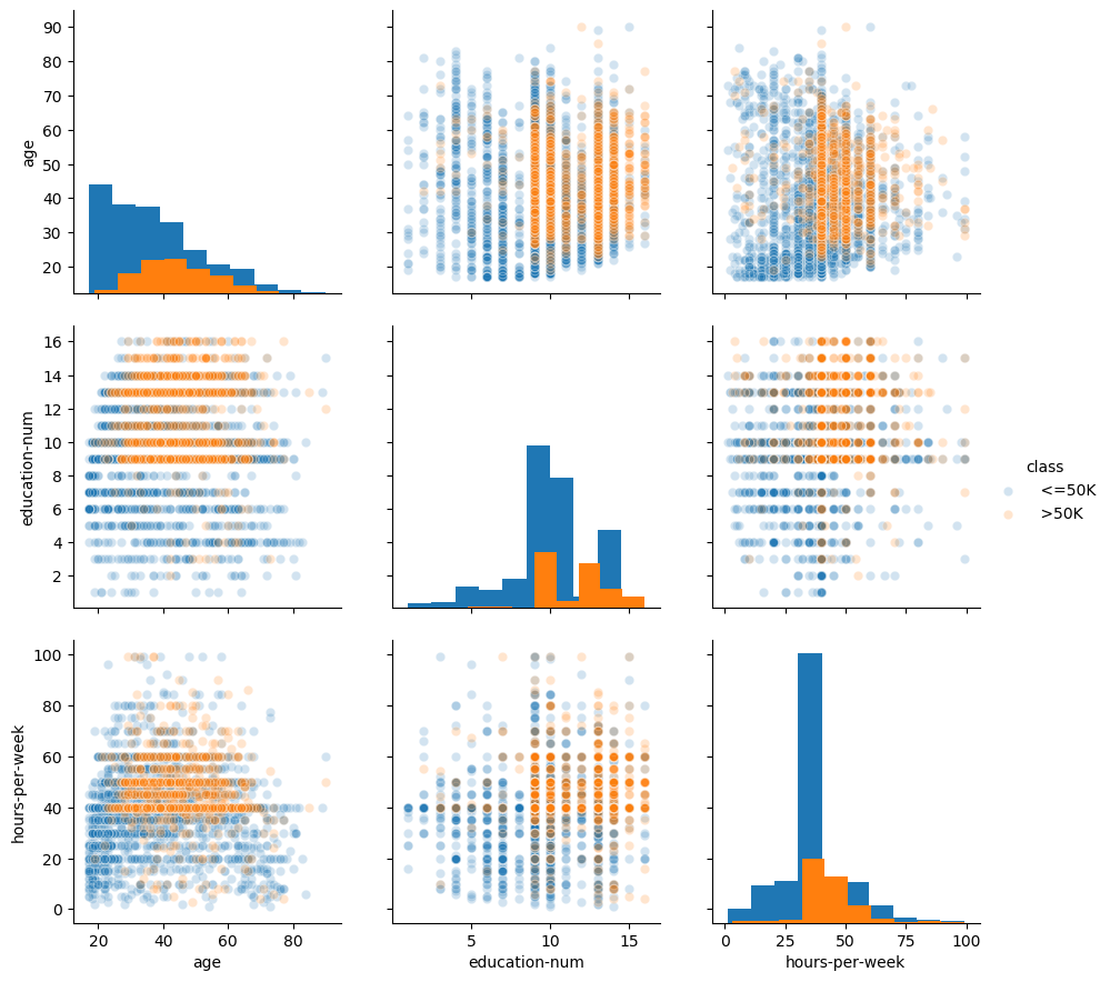
_images/01_tabular_data_exploration_28_0.png

By looking at the data you could infer some hand-written rules to predict the class:

if you are young (less than 25 year-old roughly), you are in the <= 50K class.
if you are old (more than 70 year-old roughly), you are in the <= 50K class.
if you work part-time (less than 40 hours roughly) you are in the <= 50K class.

These hand-written rules could work reasonably well without the need for any machine learning. Note however that it is not very easy to create rules for the region 40 < hours-per-week < 60 and 30 < age < 70. We can hope that machine learning can help in this region. Also note that visualization can help creating hand-written rules but is limited to 2 dimensions (maybe 3 dimensions), whereas machine learning models can build models in high-dimensional spaces.

Another thing worth mentioning in this plot: if you are young (less than 25 year-old roughly) or old (more than 70 year-old roughly) you tend to work less. This is a non-linear relationship between age and hours per week. Linear machine learning models can only capture linear interactions, so this may be a factor when deciding which model to chose.

In a machine-learning setting, an algorithm automatically create the “rules” in order to make predictions on new data.

The plot below shows the rules of a simple model, called decision tree. We will explain how this model works in a latter notebook, for now let us just consider the model predictions when trained on this dataset:

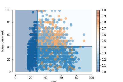
The background color in each area represents the probability of the class high-income as estimated by the model. Values towards 0 (dark blue) indicates that the model predicts low-income with a high probability. Values towards 1 (dark orange) indicates that the model predicts high-income with a high probability. Values towards 0.5 (white) indicates that the model is not very sure about its prediction.

Looking at the plot here is what we can gather:

In the region age < 28.5 (left region) the prediction is low-income. The dark blue color indicates that the model is quite sure about its prediction.
In the region age > 28.5 AND hours-per-week < 40.5 (bottom-right region), the prediction is low-income. Note that the blue is a bit lighter that for the left region which means that the algorithm is not as certain in this region.
In the region age > 28.5 AND hours-per-week > 40.5 (top-right region), the prediction is low-income. However the probability of the class low-income is very close to 0.5 which means the model is not sure at all about its prediction.

It is interesting to see that a simple model create rules similar to the ones that we could have created by hand. Note that machine learning is really interesting when creating rules by hand is not straightfoward, for example because we are in high dimension (many features) or because there is no simple and obvious rules that separate the two classes as in the top-right region

In this notebook we have:

loaded the data from a CSV file using pandas
looked at the differents kind of variables to differentiate between categorical and numerical variables
inspected the data with pandas, seaborn and pandas_profiling. Data inspection can allow you to decide whether using machine learning is appropriate for your data and to highlight potential peculiarities in your data

Ideas which will be discussed more in details later:

if your target variable is imbalanced (e.g., you have more samples from one target category than another), you may need special techniques for training and evaluating your machine learning model
having redundant (or highly correlated) columns can be a problem for some machine learning algorithms
contrary to decision tree, linear models can only capture linear interaction, so be aware of non-linear relationships in your data

Scikit-learn tutorial

Loading data into machine learning¶

Loading the adult census dataset¶

The variables (columns) in the dataset¶

Visual inspection of the data¶