First model with scikit-learn
Basic preprocessing and model fitting
In this notebook, we present how to build predictive models on tabular datasets, with numerical features. Categorical features will be discussed in the next notebook.
In particular we will highlight:
working with numerical features
the importance of scaling numerical variables
evaluate the performance of a model via cross-validation
Loading the dataset
We will use the same dataset “adult_census” described in the previous notebook. For more details about the dataset see http://www.openml.org/d/1590.
import pandas as pd

df = pd.read_csv("../datasets/adult-census.csv")
Let’s have a look at the first records of this data frame:
df.head()
| age | workclass | fnlwgt | education | education-num | marital-status | occupation | relationship | race | sex | capital-gain | capital-loss | hours-per-week | native-country | class | |
|---|---|---|---|---|---|---|---|---|---|---|---|---|---|---|---|
| 0 | 25 | Private | 226802 | 11th | 7 | Never-married | Machine-op-inspct | Own-child | Black | Male | 0 | 0 | 40 | United-States | <=50K |
| 1 | 38 | Private | 89814 | HS-grad | 9 | Married-civ-spouse | Farming-fishing | Husband | White | Male | 0 | 0 | 50 | United-States | <=50K |
| 2 | 28 | Local-gov | 336951 | Assoc-acdm | 12 | Married-civ-spouse | Protective-serv | Husband | White | Male | 0 | 0 | 40 | United-States | >50K |
| 3 | 44 | Private | 160323 | Some-college | 10 | Married-civ-spouse | Machine-op-inspct | Husband | Black | Male | 7688 | 0 | 40 | United-States | >50K |
| 4 | 18 | ? | 103497 | Some-college | 10 | Never-married | ? | Own-child | White | Female | 0 | 0 | 30 | United-States | <=50K |
target_name = "class"
target = df[target_name].to_numpy()
target
array([' <=50K', ' <=50K', ' >50K', ..., ' <=50K', ' <=50K', ' >50K'],
      dtype=object)
For simplicity, we will ignore the “fnlwgt” (final weight) column that was crafted by the creators of the dataset when sampling the dataset to be representative of the full census database.
data = df.drop(columns=[target_name, "fnlwgt"])
data.head()
| age | workclass | education | education-num | marital-status | occupation | relationship | race | sex | capital-gain | capital-loss | hours-per-week | native-country | |
|---|---|---|---|---|---|---|---|---|---|---|---|---|---|
| 0 | 25 | Private | 11th | 7 | Never-married | Machine-op-inspct | Own-child | Black | Male | 0 | 0 | 40 | United-States |
| 1 | 38 | Private | HS-grad | 9 | Married-civ-spouse | Farming-fishing | Husband | White | Male | 0 | 0 | 50 | United-States |
| 2 | 28 | Local-gov | Assoc-acdm | 12 | Married-civ-spouse | Protective-serv | Husband | White | Male | 0 | 0 | 40 | United-States |
| 3 | 44 | Private | Some-college | 10 | Married-civ-spouse | Machine-op-inspct | Husband | Black | Male | 7688 | 0 | 40 | United-States |
| 4 | 18 | ? | Some-college | 10 | Never-married | ? | Own-child | White | Female | 0 | 0 | 30 | United-States |
Working with numerical data
Numerical data is the most natural type of data used in machine learning and can (almost) directly be fed to predictive models. We can quickly have a look at such data by selecting the subset of numerical columns from the original data.
We will use this subset of data to fit a linear classification model to predict the income class.
data.columns
Index(['age', 'workclass', 'education', 'education-num', 'marital-status',
       'occupation', 'relationship', 'race', 'sex', 'capital-gain',
       'capital-loss', 'hours-per-week', 'native-country'],
      dtype='object')
data.dtypes
age                int64
workclass         object
education         object
education-num      int64
marital-status    object
occupation        object
relationship      object
race              object
sex               object
capital-gain       int64
capital-loss       int64
hours-per-week     int64
native-country    object
dtype: object
from sklearn.compose import make_column_selector as selector

numerical_columns_selector = selector(dtype_include=["int", "float"])
numerical_columns = numerical_columns_selector(data)
numerical_columns
['age', 'education-num', 'capital-gain', 'capital-loss', 'hours-per-week']
data_numeric = data[numerical_columns]
data_numeric.head()
| age | education-num | capital-gain | capital-loss | hours-per-week | |
|---|---|---|---|---|---|
| 0 | 25 | 7 | 0 | 0 | 40 |
| 1 | 38 | 9 | 0 | 0 | 50 |
| 2 | 28 | 12 | 0 | 0 | 40 |
| 3 | 44 | 10 | 7688 | 0 | 40 |
| 4 | 18 | 10 | 0 | 0 | 30 |
When building a machine learning model, it is important to leave out a subset of the data which we can use later to evaluate the trained model. The data used to fit a model is called training data while the one used to assess a model is called testing data.
Scikit-learn provides a helper function train_test_split which will
split the dataset into a training and a testing set. It will also ensure that
the data are shuffled randomly before splitting the data.
from sklearn.model_selection import train_test_split

data_train, data_test, target_train, target_test = train_test_split(
    data_numeric, target, random_state=42)
print(
    f"The training dataset contains {data_train.shape[0]} samples and "
    f"{data_train.shape[1]} features")
The training dataset contains 36631 samples and 5 features
print(
    f"The testing dataset contains {data_test.shape[0]} samples and "
    f"{data_test.shape[1]} features")
The testing dataset contains 12211 samples and 5 features
We will build a linear classification model called “Logistic Regression”. The
fit method is called to train the model from the input (features) and
target data. Only the training data should be given for this purpose.
In addition, check the time required to train the model and the number of iterations done by the solver to find a solution.
from sklearn.linear_model import LogisticRegression
import time

model = LogisticRegression()
start = time.time()
model.fit(data_train, target_train)
elapsed_time = time.time() - start

print(f"The model {model.__class__.__name__} was trained in "
      f"{elapsed_time:.3f} seconds for {model.n_iter_} iterations")
The model LogisticRegression was trained in 0.368 seconds for [100] iterations
/home/lesteve/miniconda3/envs/scikit-learn-tutorial/lib/python3.7/site-packages/sklearn/linear_model/_logistic.py:764: ConvergenceWarning: lbfgs failed to converge (status=1):
STOP: TOTAL NO. of ITERATIONS REACHED LIMIT.

Increase the number of iterations (max_iter) or scale the data as shown in:
    https://scikit-learn.org/stable/modules/preprocessing.html
Please also refer to the documentation for alternative solver options:
    https://scikit-learn.org/stable/modules/linear_model.html#logistic-regression
  extra_warning_msg=_LOGISTIC_SOLVER_CONVERGENCE_MSG)
Let’s ignore the convergence warning for now and instead let’s try to use our model to make some predictions on the first five records of the held out test set:
target_predicted = model.predict(data_test)
target_predicted[:5]
array([' <=50K', ' <=50K', ' >50K', ' <=50K', ' <=50K'], dtype=object)
target_test[:5]
array([' <=50K', ' <=50K', ' >50K', ' <=50K', ' <=50K'], dtype=object)
predictions = data_test.copy()
predictions['predicted-class'] = target_predicted
predictions['expected-class'] = target_test
predictions['correct'] = target_predicted == target_test
predictions.head()
| age | education-num | capital-gain | capital-loss | hours-per-week | predicted-class | expected-class | correct | |
|---|---|---|---|---|---|---|---|---|
| 7762 | 56 | 9 | 0 | 0 | 40 | <=50K | <=50K | True |
| 23881 | 25 | 9 | 0 | 0 | 40 | <=50K | <=50K | True |
| 30507 | 43 | 13 | 14344 | 0 | 40 | >50K | >50K | True |
| 28911 | 32 | 9 | 0 | 0 | 40 | <=50K | <=50K | True |
| 19484 | 39 | 13 | 0 | 0 | 30 | <=50K | <=50K | True |
To quantitatively evaluate our model, we can use the method score. It will
compute the classification accuracy when dealing with a classification
problem.
print(f"The test accuracy using a {model.__class__.__name__} is "
      f"{model.score(data_test, target_test):.3f}")
The test accuracy using a LogisticRegression is 0.818
This is mathematically equivalent as computing the average number of time the model makes a correct prediction on the test set:
(target_test == target_predicted).mean()
0.8177053476373761
Exercise 1
What would be the score of a model that always predicts
' >50K'?What would be the score of a model that always predicts
' <= 50K'?Is 81% or 82% accuracy a good score for this problem?
Hint: You can use a DummyClassifier and do a train-test split to evaluate
its accuracy on the test set. This
link
shows a few examples of how to evaluate the performance of these baseline
models.
Open the dedicated notebook in Jupyter to do this exercise.
Let’s now consider the ConvergenceWarning message that was raised previously
when calling the fit method to train our model. This warning informs us that
our model stopped learning because it reached the maximum number of
iterations allowed by the user. This could potentially be detrimental for the
model accuracy. We can follow the (bad) advice given in the warning message
and increase the maximum number of iterations allowed.
model = LogisticRegression(max_iter=50000)
start = time.time()
model.fit(data_train, target_train)
elapsed_time = time.time() - start
print(
    f"The accuracy using a {model.__class__.__name__} is "
    f"{model.score(data_test, target_test):.3f} with a fitting time of "
    f"{elapsed_time:.3f} seconds in {model.n_iter_} iterations")
The accuracy using a LogisticRegression is 0.818 with a fitting time of 0.372 seconds in [105] iterations
We now observe a longer training time but no significant improvement in the predictive performance. Instead of increasing the number of iterations, we can try to help fit the model faster by scaling the data first. A range of preprocessing algorithms in scikit-learn allows us to transform the input data before training a model.
In our case, we will standardize the data and then train a new logistic regression model on that new version of the dataset.
data_train.describe()
| age | education-num | capital-gain | capital-loss | hours-per-week | |
|---|---|---|---|---|---|
| count | 36631.000000 | 36631.000000 | 36631.000000 | 36631.000000 | 36631.000000 |
| mean | 38.642352 | 10.078131 | 1087.077721 | 89.665311 | 40.431247 |
| std | 13.725748 | 2.570143 | 7522.692939 | 407.110175 | 12.423952 |
| min | 17.000000 | 1.000000 | 0.000000 | 0.000000 | 1.000000 |
| 25% | 28.000000 | 9.000000 | 0.000000 | 0.000000 | 40.000000 |
| 50% | 37.000000 | 10.000000 | 0.000000 | 0.000000 | 40.000000 |
| 75% | 48.000000 | 12.000000 | 0.000000 | 0.000000 | 45.000000 |
| max | 90.000000 | 16.000000 | 99999.000000 | 4356.000000 | 99.000000 |
from sklearn.preprocessing import StandardScaler

scaler = StandardScaler()
data_train_scaled = scaler.fit_transform(data_train)
data_train_scaled
array([[ 0.17177061,  0.35868902, -0.14450843,  5.71188483, -2.28845333],
       [ 0.02605707,  1.1368665 , -0.14450843, -0.22025127, -0.27618374],
       [-0.33822677,  1.1368665 , -0.14450843, -0.22025127,  0.77019645],
       ...,
       [-0.77536738, -0.03039972, -0.14450843, -0.22025127, -0.03471139],
       [ 0.53605445,  0.35868902, -0.14450843, -0.22025127, -0.03471139],
       [ 1.48319243,  1.52595523, -0.14450843, -0.22025127, -2.69090725]])
data_train_scaled = pd.DataFrame(data_train_scaled,
                                 columns=data_train.columns)
data_train_scaled.describe()
| age | education-num | capital-gain | capital-loss | hours-per-week | |
|---|---|---|---|---|---|
| count | 3.663100e+04 | 3.663100e+04 | 3.663100e+04 | 3.663100e+04 | 3.663100e+04 |
| mean | -2.273364e-16 | 1.219606e-16 | 3.530310e-17 | 3.840667e-17 | 1.844684e-16 |
| std | 1.000014e+00 | 1.000014e+00 | 1.000014e+00 | 1.000014e+00 | 1.000014e+00 |
| min | -1.576792e+00 | -3.532198e+00 | -1.445084e-01 | -2.202513e-01 | -3.173852e+00 |
| 25% | -7.753674e-01 | -4.194885e-01 | -1.445084e-01 | -2.202513e-01 | -3.471139e-02 |
| 50% | -1.196565e-01 | -3.039972e-02 | -1.445084e-01 | -2.202513e-01 | -3.471139e-02 |
| 75% | 6.817680e-01 | 7.477778e-01 | -1.445084e-01 | -2.202513e-01 | 3.677425e-01 |
| max | 3.741752e+00 | 2.304133e+00 | 1.314865e+01 | 1.047970e+01 | 4.714245e+00 |
We can easily combine these sequential operations
with a scikit-learn Pipeline, which chains together operations and can be
used like any other classifier or regressor. The helper function
make_pipeline will create a Pipeline by giving as arguments the successive
transformations to perform followed by the classifier or regressor model.
from sklearn.pipeline import make_pipeline

model = make_pipeline(StandardScaler(),
                      LogisticRegression())
start = time.time()
model.fit(data_train, target_train)
elapsed_time = time.time() - start
print(
    f"The accuracy using a {model.__class__.__name__} is "
    f"{model.score(data_test, target_test):.3f} with a fitting time of "
    f"{elapsed_time:.3f} seconds in {model[-1].n_iter_} iterations")
The accuracy using a Pipeline is 0.818 with a fitting time of 0.089 seconds in [13] iterations
We can see that the training time and the number of iterations is much shorter while the predictive performance (accuracy) stays the same.
In the previous example, we split the original data into a training set and a testing set. This strategy has several issues: in the setting where the amount of data is limited, the subset of data used to train or test will be small; and the splitting was done in a random manner and we have no information regarding the confidence of the results obtained.
Instead, we can use cross-validation. Cross-validation consists of repeating this random splitting into training and testing sets and aggregating the model performance. By repeating the experiment, one can get an estimate of the variability of the model performance.
The function cross_val_score allows for such experimental protocol by giving
the model, the data and the target. Since there exists several
cross-validation strategies, cross_val_score takes a parameter cv which
defines the splitting strategy.
%%time
from sklearn.model_selection import cross_val_score

scores = cross_val_score(model, data_numeric, target, cv=5)
CPU times: user 1.19 s, sys: 23.9 ms, total: 1.21 s
Wall time: 607 ms
scores
array([0.81216092, 0.8096018 , 0.81337019, 0.81326781, 0.82207207])
print(f"The mean cross-validation accuracy is: "
      f"{scores.mean():.3f} +/- {scores.std():.3f}")
The mean cross-validation accuracy is: 0.814 +/- 0.004
Note that by computing the standard-deviation of the cross-validation scores we can get an idea of the uncertainty of our estimation of the predictive performance of the model: in the above results, only the first 2 decimals seem to be trustworthy. Using a single train / test split would not allow us to know anything about the level of uncertainty of the accuracy of the model.
Setting cv=5 created 5 distinct splits to get 5 variations for the training
and testing sets. Each training set is used to fit one model which is then
scored on the matching test set. This strategy is called K-fold
cross-validation where K corresponds to the number of splits.
The figure helps visualize how the dataset is partitioned into train and test samples at each iteration of the cross-validation procedure:
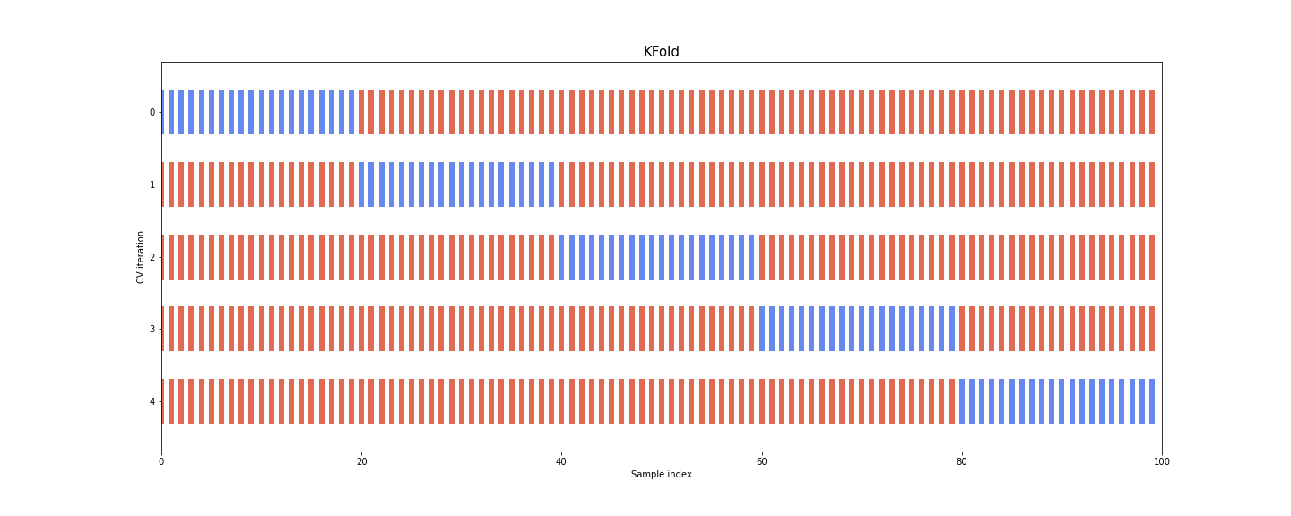
For each cross-validation split, the procedure trains a model on the concatenation of the red samples and evaluate the score of the model by using the blue samples. Cross-validation is therefore computationally intensive because it requires training several models instead of one.
Note that the cross_val_score method above discards the 5 models that
were trained on the different overlapping subset of the dataset.
The goal of cross-validation is not to train a model, but rather to
estimate approximately the generalization performance of a model that
would have been trained to the full training set, along with an estimate
of the variability (uncertainty on the generalization accuracy).
In this notebook we have:
split our dataset into a training dataset and a testing dataset
fitted a logistic regression model
seen the importance of scaling numerical variables
used the pipeline method to fit both the scaler and the logistic regression
assessed the performance of our model via cross-validation