Linear Models¶

In this notebook we will review linear models from scikit-learn. We will :

learn how to fit a simple linear model and interpret the coefficients;
discuss feature augmentation to fit a non-linear function;
use LinearRegression and its regularized version Ridge which is more robust;
use LogisticRegression with pipeline;
see examples of linear separability.

1. Regression¶

The over-simplistic toy example¶

To illustrate the main principle of linear regression, we will use a dataset that contains information about penguins.

import pandas as pd

data = pd.read_csv("../datasets/penguins.csv")
data.head()

	studyName	Sample Number	Species	Region	Island	Stage	Individual ID	Clutch Completion	Date Egg	Culmen Length (mm)	Culmen Depth (mm)	Flipper Length (mm)	Body Mass (g)	Sex	Delta 15 N (o/oo)	Delta 13 C (o/oo)	Comments
0	PAL0708	1	Adelie Penguin (Pygoscelis adeliae)	Anvers	Torgersen	Adult, 1 Egg Stage	N1A1	Yes	2007-11-11	39.1	18.7	181.0	3750.0	MALE	NaN	NaN	Not enough blood for isotopes.
1	PAL0708	2	Adelie Penguin (Pygoscelis adeliae)	Anvers	Torgersen	Adult, 1 Egg Stage	N1A2	Yes	2007-11-11	39.5	17.4	186.0	3800.0	FEMALE	8.94956	-24.69454	NaN
2	PAL0708	3	Adelie Penguin (Pygoscelis adeliae)	Anvers	Torgersen	Adult, 1 Egg Stage	N2A1	Yes	2007-11-16	40.3	18.0	195.0	3250.0	FEMALE	8.36821	-25.33302	NaN
3	PAL0708	4	Adelie Penguin (Pygoscelis adeliae)	Anvers	Torgersen	Adult, 1 Egg Stage	N2A2	Yes	2007-11-16	NaN	NaN	NaN	NaN	NaN	NaN	NaN	Adult not sampled.
4	PAL0708	5	Adelie Penguin (Pygoscelis adeliae)	Anvers	Torgersen	Adult, 1 Egg Stage	N3A1	Yes	2007-11-16	36.7	19.3	193.0	3450.0	FEMALE	8.76651	-25.32426	NaN

This dataset contains measurements taken of penguins. We will formulate the following problem: using the flipper length of a penguin, we would like to infer its mass.

import seaborn as sns

feature_names = "Flipper Length (mm)"
target_name = "Body Mass (g)"

sns.scatterplot(data=data, x=feature_names, y=target_name)

# select the features of interest
X = data[[feature_names]].dropna()
y = data[target_name].dropna()

In this problem, penguin mass is our target. It is a continuous variable that roughly varies between 2700 g and 6300 g. Thus, this is a regression problem (in contrast to classification). We also see that there is almost a linear relationship between the body mass of the penguin and the flipper length. The longer the flipper, the heavier the penguin.

Thus, we could come up with a simple formula, where given a flipper length we could compute the body mass of a penguin using a linear relationship of of the form y = a * x + b where a and b are the 2 parameters of our model.

def linear_model_flipper_mass(
    flipper_length, weight_flipper_length, intercept_body_mass
):
    """Linear model of the form y = a * x + b"""
    body_mass = weight_flipper_length * flipper_length + intercept_body_mass
    return body_mass

Using the model we defined above, we can check the body mass values predicted for a range of flipper lengths. We will set weight_flipper_length to be 45 and intercept_body_mass to be -5000.

import matplotlib.pyplot as plt
import numpy as np


def plot_data_and_model(
    flipper_length_range, weight_flipper_length, intercept_body_mass,
    ax=None,
):
    """Compute and plot the prediction."""
    inferred_body_mass = linear_model_flipper_mass(
        flipper_length_range,
        weight_flipper_length=weight_flipper_length,
        intercept_body_mass=intercept_body_mass,
    )

    if ax is None:
        _, ax = plt.subplots()

    sns.scatterplot(data=data, x=feature_names, y=target_name, ax=ax)
    ax.plot(
        flipper_length_range,
        inferred_body_mass,
        linewidth=3,
        label=(
            f"{weight_flipper_length:.2f} (g / mm) * flipper length + "
            f"{intercept_body_mass:.2f} (g)"
        ),
    )
    plt.legend()


weight_flipper_length = 45
intercept_body_mass = -5000

flipper_length_range = np.linspace(X.min(), X.max(), num=300)
plot_data_and_model(
    flipper_length_range, weight_flipper_length, intercept_body_mass
)

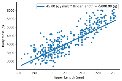
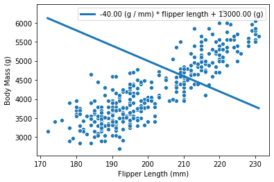
The variable weight_flipper_length is a weight applied to the feature flipper_length in order to make the inference. When this coefficient is positive, it means that penguins with longer flipper lengths will have larger body masses. If the coefficient is negative, it means that penguins with shorter flipper flipper lengths have larger body masses. Graphically, this coefficient is represented by the slope of the curve in the plot. Below we show what the curve would look like when the weight_flipper_length coefficient is negative.

weight_flipper_length = -40
intercept_body_mass = 13000

flipper_length_range = np.linspace(X.min(), X.max(), num=300)
plot_data_and_model(
    flipper_length_range, weight_flipper_length, intercept_body_mass
)

In our case, this coefficient has a meaningful unit: g/mm. For instance, a coefficient of 40 g/mm, means that for each additional millimeter in flipper length, the body weight predicted will increase by 40 g.

body_mass_180 = linear_model_flipper_mass( flipper_length=180, weight_flipper_length=40, intercept_body_mass=0 ) body_mass_181 = linear_model_flipper_mass( flipper_length=181, weight_flipper_length=40, intercept_body_mass=0 )

print( f”The body mass for a flipper length of 180 mm is {body_mass_180} g and “ f”{body_mass_181} g for a flipper length of 181 mm” )

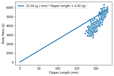
We can also see that we have a parameter intercept_body_mass in our model. This parameter corresponds to the value on the y-axis if flipper_length=0 (which in our case is only a mathematical consideration, as in our data, the value of flipper_length only goes from 170mm to 230mm). This y-value when
x=0 is called the y-intercept. If intercept_body_mass is 0, the curve will pass through the origin:

weight_flipper_length = 25
intercept_body_mass = 0

flipper_length_range = np.linspace(0, X.max(), num=300)
plot_data_and_model(
    flipper_length_range, weight_flipper_length, intercept_body_mass
)

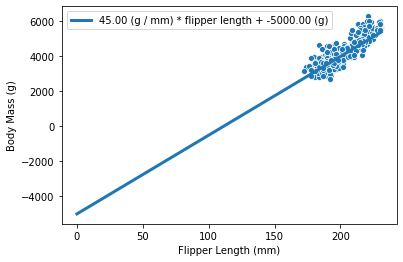
Otherwise, it will pass through the intercept_body_mass value:

weight_flipper_length = 45
intercept_body_mass = -5000

flipper_length_range = np.linspace(0, X.max(), num=300)
plot_data_and_model(
    flipper_length_range, weight_flipper_length, intercept_body_mass
)

Now, that we understand how our model is inferring data, one should ask how do we find the best value for the parameters. Indeed, it seems that we can have many models, depending of the choice of parameters:

_, ax = plt.subplots()
flipper_length_range = np.linspace(X.min(), X.max(), num=300)
for weight, intercept in zip([-40, 45, 90], [15000, -5000, -14000]):
    plot_data_and_model(
        flipper_length_range, weight, intercept, ax=ax,
    )

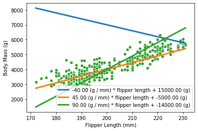
To choose a model, we could use a metric that indicates how good our model is at fitting our data.

from sklearn.metrics import mean_squared_error

for weight, intercept in zip([-40, 45, 90], [15000, -5000, -14000]):
    inferred_body_mass = linear_model_flipper_mass(
        X,
        weight_flipper_length=weight,
        intercept_body_mass=intercept,
    )
    model_error = mean_squared_error(y, inferred_body_mass)
    print(
        f"The following model \n "
        f"{weight:.2f} (g / mm) * flipper length + {intercept:.2f} (g) \n"
        f"has a mean squared error of: {model_error:.2f}"
    )

The following model 
 -40.00 (g / mm) * flipper length + 15000.00 (g) 
has a mean squared error of: 9366992.84
The following model 
 45.00 (g / mm) * flipper length + -5000.00 (g) 
has a mean squared error of: 184657.38
The following model 
 90.00 (g / mm) * flipper length + -14000.00 (g) 
has a mean squared error of: 489223.83

Thus, the best model will be the one with the lowest error. Hopefully, this problem of finding the best parameters values (i.e. that result in the lowest error) can be solved without the need to check every potential parameter combination. Indeed, this problem has a closed-form solution: the best parameter values can be found by solving an equation. This avoids the need for brute-force search. This strategy is implemented in scikit-learn.

from sklearn.linear_model import LinearRegression

linear_regression = LinearRegression()
linear_regression.fit(X, y)

LinearRegression()

The instance linear_regression will store the parameter values in the attributes coef_ and intercept_. We can check what the optimal model found is:

weight_flipper_length = linear_regression.coef_[0]
intercept_body_mass = linear_regression.intercept_

flipper_length_range = np.linspace(X.min(), X.max(), num=300)
plot_data_and_model(
    flipper_length_range, weight_flipper_length, intercept_body_mass
)

inferred_body_mass = linear_regression.predict(X)
model_error = mean_squared_error(y, inferred_body_mass)
print(f"The error of the optimal model is {model_error:.2f}")

The error of the optimal model is 154546.19

What if your data doesn’t have a linear relationship¶

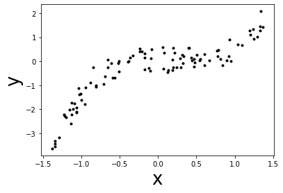
Now, we will define a new problem where the feature and the target are not linearly linked. For instance, we could define x to be the years of experience (normalized) and y the salary (normalized). Therefore, the problem here would be to infer the salary given the years of experience.

# data generation
# fix the seed for reproduction
rng = np.random.RandomState(0)

n_sample = 100
x_max, x_min = 1.4, -1.4
len_x = (x_max - x_min)
x = rng.rand(n_sample) * len_x - len_x/2
noise = rng.randn(n_sample) * .3
y = x ** 3 - 0.5 * x ** 2 + noise

# plot the data
plt.scatter(x, y,  color='k', s=9)
plt.xlabel('x', size=26)
_ = plt.ylabel('y', size=26)

Exercise 1¶

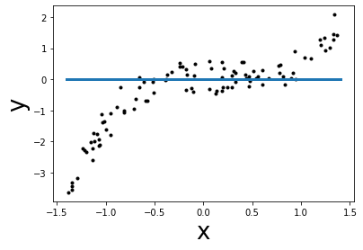
In this exercise, you are asked to approximate the target y using a linear function f(x). i.e. find the best coefficients of the function f in order to minimize the mean squared error. Here you shall find the coefficient manually via trial and error (just as in the previous cells with weight and intercept).

Then you can compare the mean squared error of your model with the mean squared error found by LinearRegression (which shall be the minimal one).

def f(x):
    intercept = 0  # TODO: update the parameters here
    weight = 0  # TODO: update the parameters here
    y_predict = weight * x + intercept
    return y_predict


# plot the slope of f
grid = np.linspace(x_min, x_max, 300)
plt.scatter(x, y, color='k', s=9)
plt.plot(grid, f(grid), linewidth=3)
plt.xlabel("x", size=26)
plt.ylabel("y", size=26)

mse = mean_squared_error(y, f(x))
print(f"Mean squared error = {mse:.2f}")

Mean squared error = 1.53

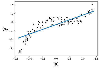
Solution 1. by fiting a linear regression¶

from sklearn import linear_model

linear_regression = linear_model.LinearRegression()
# X should be 2D for sklearn
X = x.reshape((-1, 1))
linear_regression.fit(X, y)

# plot the best slope
y_best = linear_regression.predict(grid.reshape(-1, 1))
plt.plot(grid, y_best, linewidth=3)
plt.scatter(x, y, color="k", s=9)
plt.xlabel("x", size=26)
plt.ylabel("y", size=26)

mse = mean_squared_error(y, linear_regression.predict(X))
print(f"Lowest mean squared error = {mse:.2f}")

Lowest mean squared error = 0.37

Here the coefficients learnt by LinearRegression is the best curve that fits the data. We can inspect the coefficients using the attributes of the model learnt as follows:

print(
    f"best coef: w1 = {linear_regression.coef_[0]:.2f}, "
    f"best intercept: w0 = {linear_regression.intercept_:.2f}"
)

best coef: w1 = 1.25, best intercept: w0 = -0.29

It is important to note that the model learnt will not be able to handle the non-linear relationship between x and y since linear models assume the relationship between x and y to be linear. To obtain a better model, we have 3 main solutions:

choose a model that natively can deal with non-linearity,
“augment” features by including expert knowledge which can be used by the model, or
use a “kernel” to have a locally-based decision function instead of a global linear decision function.

Let’s illustrate quickly the first point by using a decision tree regressor which can natively handle non-linearity.

from sklearn.tree import DecisionTreeRegressor

tree = DecisionTreeRegressor(max_depth=3).fit(X, y)
y_pred = tree.predict(grid.reshape(-1, 1))

plt.plot(grid, y_pred, linewidth=3)
plt.scatter(x, y, color="k", s=9)
plt.xlabel("x", size=26)
plt.ylabel("y", size=26)

mse = mean_squared_error(y, tree.predict(X))
print(f"Lowest mean squared error = {mse:.2f}")

Lowest mean squared error = 0.09

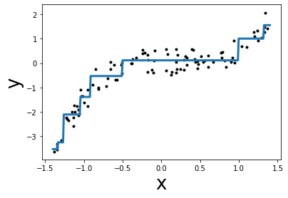
In this case, the model can handle non-linearity. Instead of having a model which can natively deal with non-linearity, we could also modify our data: we could create new features, derived from the original features, using some expert knowledge. For instance, here we know that we have a cubic and squared relationship between x and y (because we generated the data). Indeed, we could create two new features (x^2 and x^3) using this information.

X = np.vstack([x, x ** 2, x ** 3]).T

linear_regression.fit(X, y)

grid_augmented = np.vstack([grid, grid ** 2, grid ** 3]).T
y_pred = linear_regression.predict(grid_augmented)

plt.plot(grid, y_pred, linewidth=3)
plt.scatter(x, y, color="k", s=9)
plt.xlabel("x", size=26)
plt.ylabel("y", size=26)

mse = mean_squared_error(y, linear_regression.predict(X))
print(f"Lowest mean squared error = {mse:.2f}")

Lowest mean squared error = 0.09

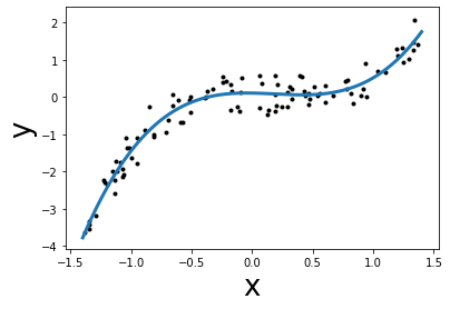
We can see that even with a linear model, we can overcome the linearity limitation of the model by adding the non-linear component into the design of additional features. Here, we created new feature by knowing the way the target was generated. In practice, this is usually not the case. Instead, one is usually creating interaction between features (e.g. \(x_1 * x_2\)) with different orders (e.g. \(x_1, x_1^2, x_1^3\)), at the risk of creating a model with too much expressivity and which might overfit. In scikit-learn, the PolynomialFeatures is a transformer to create such feature interactions which we could have used instead of manually creating new features.

To demonstrate PolynomialFeatures, we are going to use a scikit-learn pipeline which will first create the new features and then fit the model. We come back to scikit-learn pipelines and discuss them in more detail later.

from sklearn.pipeline import make_pipeline
from sklearn.preprocessing import PolynomialFeatures

X = x.reshape(-1, 1)

model = make_pipeline(
    PolynomialFeatures(degree=3), LinearRegression()
)
model.fit(X, y)
y_pred = model.predict(grid.reshape(-1, 1))

plt.plot(grid, y_pred, linewidth=3)
plt.scatter(x, y, color="k", s=9)
plt.xlabel("x", size=26)
plt.ylabel("y", size=26)

mse = mean_squared_error(y, model.predict(X))
print(f"Lowest mean squared error = {mse:.2f}")

Lowest mean squared error = 0.09

Thus, we saw that PolynomialFeatures is actually doing the same operation that we did manually above.

FIXME: it might be to complex to be introduced here but it seems good in the flow. However, we go away from linear model.

The last possibility to make a linear model more expressive is to use a “kernel”. Instead of learning a weight per feature as we previously emphasized, a weight will be assign by sample instead. However, not all samples will be used. This is the base of the support vector machine algorithm.

from sklearn.svm import SVR

svr = SVR(kernel="linear").fit(X, y)
y_pred = svr.predict(grid.reshape(-1, 1))

plt.plot(grid, y_pred, linewidth=3)
plt.scatter(x, y, color="k", s=9)
plt.xlabel("x", size=26)
plt.ylabel("y", size=26)

mse = mean_squared_error(y, svr.predict(X))
print(f"Lowest mean squared error = {mse:.2f}")

Lowest mean squared error = 0.38

The algorithm can be modified such that it can use non-linear kernel. Then, it will compute interaction between samples using this non-linear interaction.

svr = SVR(kernel=”poly”, degree=3).fit(X, y) y_pred = svr.predict(grid.reshape(-1, 1))

plt.plot(grid, y_pred, linewidth=3) plt.scatter(x, y, color=”k”, s=9) plt.xlabel(“x”, size=26) plt.ylabel(“y”, size=26)

mse = mean_squared_error(y, svr.predict(X)) print(f”Lowest mean squared error = {mse:.2f}”)

Therefore, kernel can make a model more expressive.

Linear regression in higher dimension¶

In the previous example, we only used a single feature. But we have already shown that we could add new feature to make the model more expressive by deriving new features, based on the original feature.

Indeed, we could also use additional features (not related to the original feature) and these could help us to predict the target.

We will load a dataset about house prices in California. The dataset consists of 8 features regarding the demography and geography of districts in California and the aim is to predict the median house price of each district. We will use all 8 features to predict the target, median house price.

from sklearn.datasets import fetch_california_housing

X, y = fetch_california_housing(as_frame=True, return_X_y=True)
X.head()

	MedInc	HouseAge	AveRooms	AveBedrms	Population	AveOccup	Latitude	Longitude
0	8.3252	41.0	6.984127	1.023810	322.0	2.555556	37.88	-122.23
1	8.3014	21.0	6.238137	0.971880	2401.0	2.109842	37.86	-122.22
2	7.2574	52.0	8.288136	1.073446	496.0	2.802260	37.85	-122.24
3	5.6431	52.0	5.817352	1.073059	558.0	2.547945	37.85	-122.25
4	3.8462	52.0	6.281853	1.081081	565.0	2.181467	37.85	-122.25

We will compare the score of LinearRegression and Ridge (which is a regularized version of linear regression).

The scorer we will use to evaluate our model is the mean squared error, as in the previous example. The lower the score, the better.

Here, we will divide our data into a training set, a validation set and a testing set. The validation set will be used to evaluate selection of the hyper-parameters, while the testing set should only be used to calculate the score of our final model.

from sklearn.model_selection import train_test_split

X_train_valid, X_test, y_train_valid, y_test = train_test_split(
    X, y, random_state=1
)

X_train, X_valid, y_train, y_valid = train_test_split(
    X_train_valid, y_train_valid, random_state=1
)

Note that in the first example, we did not care about scaling our data in order to keep the original units and have better intuition. However, it is good practice to scale the data such that each feature has a similar standard deviation. It will be even more important if the solver used by the model is a gradient-descent-based solver.

from sklearn.preprocessing import StandardScaler

scaler = StandardScaler()
X_train_scaled = scaler.fit(X_train).transform(X_train)
X_valid_scaled = scaler.transform(X_valid)

Scikit-learn provides several tools to preprocess the data. The StandardScaler transforms the data such that each feature will have a mean of zero and a standard deviation of 1.

This scikit-learn estimator is known as a transformer: it computes some statistics (i.e the mean and the standard deviation) and stores them as attributes (scaler.mean_, scaler.scale_) when calling fit. Using these statistics, it transform the data when transform is called. Therefore, it is important to note that fit should only be called on the training data, similar to classifiers and regressors.

print('mean records on the training set:', scaler.mean_)
print('standard deviation records on the training set:', scaler.scale_)

mean records on the training set: [ 3.88516817e+00  2.85975022e+01  5.43642135e+00  1.09589237e+00
  1.42820345e+03  3.10666017e+00  3.56320086e+01 -1.19577850e+02]
standard deviation records on the training set: [1.90337997e+00 1.25434100e+01 2.37294735e+00 4.64651062e-01
 1.13564841e+03 1.26469009e+01 2.13361408e+00 2.00827882e+00]

In the example above, X_train_scaled is the data scaled, using the mean and standard deviation of each feature, computed using the training data X_train.

linear_regression = LinearRegression()
linear_regression.fit(X_train_scaled, y_train)
y_pred = linear_regression.predict(X_valid_scaled)
print(
    f"Mean squared error on the validation set: "
    f"{mean_squared_error(y_valid, y_pred):.4f}"
)

Mean squared error on the validation set: 0.5085

Instead of calling the transformer to transform the data and then calling the regressor, scikit-learn provides a Pipeline, which ‘chains’ the transformer and regressor together. The pipeline allows you to use a sequence of transformer(s) followed by a regressor or a classifier, in one call. (i.e. fitting the pipeline will fit both the transformer(s) and the regressor. Then predicting from the pipeline will first transform the data through the transformer(s) then predict with the regressor from the transformed data)

This pipeline exposes the same API as the regressor and classifier and will manage the calls to fit and transform for you, avoiding any problems with data leakage (when knowledge of the test data was inadvertently included in training a model, as when fitting a transformer on the test data).

We already presented Pipeline in the second notebook and we will use it here to combine both the scaling and the linear regression.

We will can create a Pipeline by using make_pipeline and giving as arguments the transformation(s) to be performed (in order) and the regressor model.

So the two cells above can be reduced to this new one:

from sklearn.pipeline import make_pipeline

linear_regression = make_pipeline(StandardScaler(), LinearRegression())

linear_regression.fit(X_train, y_train)
y_pred_valid = linear_regression.predict(X_valid)
linear_regression_score = mean_squared_error(y_valid, y_pred_valid)
y_pred_test = linear_regression.predict(X_test)

print(
    f"Mean squared error on the validation set: "
    f"{mean_squared_error(y_valid, y_pred_valid):.4f}"
)
print(
    f"Mean squared error on the test set: "
    f"{mean_squared_error(y_test, y_pred_test):.4f}"
)

Mean squared error on the validation set: 0.5085
Mean squared error on the test set: 0.5361

Now we want to compare this basic LinearRegression versus its regularized form Ridge.

We will tune the parameter alpha in Ridge and compare the results with the LinearRegression model which is not regularized.

from sklearn.linear_model import Ridge

ridge = make_pipeline(StandardScaler(), Ridge())

list_alphas = np.logspace(-2, 2.1, num=40)
list_ridge_scores = []
for alpha in list_alphas:
    ridge.set_params(ridge__alpha=alpha)
    ridge.fit(X_train, y_train)
    y_pred = ridge.predict(X_valid)
    list_ridge_scores.append(mean_squared_error(y_valid, y_pred))

plt.plot(
    list_alphas, [linear_regression_score] * len(list_alphas), '--',
    label='LinearRegression',
)
plt.plot(list_alphas, list_ridge_scores, "+-", label='Ridge')
plt.xlabel('alpha (regularization strength)')
plt.ylabel('Mean squared error (lower is better')
_ = plt.legend()

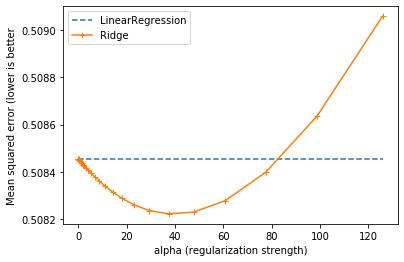
We see that, just like adding salt in cooking, adding regularization in our model could improve its error on the validation set. But too much regularization, like too much salt, decreases its performance.

We can see visually that the best alpha should be around 40.

best_alpha = list_alphas[np.argmin(list_ridge_scores)]
best_alpha

37.528307143701745

Note that, we selected this alpha without using the testing set ; but instead by using the validation set which is a subset of the training data. This is so we do not “overfit” the test data and can be seen in the lesson basic hyper-parameters tuning. We can finally compare the performance of the LinearRegression model to the best Ridge model, on the testing set.

print("Linear Regression")
y_pred_test = linear_regression.predict(X_test)
print(
    f"Mean squared error on the test set: "
    f"{mean_squared_error(y_test, y_pred_test):.4f}"
)

print("Ridge Regression")
ridge.set_params(ridge__alpha=alpha)
ridge.fit(X_train, y_train)
y_pred_test = ridge.predict(X_test)
print(
    f"Mean squared error on the test set: "
    f"{mean_squared_error(y_test, y_pred_test):.4f}"
)
# FIXME add explication why Ridge is not better (equivalent) than linear 
# regression here.

Linear Regression
Mean squared error on the test set: 0.5361
Ridge Regression
Mean squared error on the test set: 0.5367

The hyper-parameter search could have been made using GridSearchCV instead of manually splitting the training data (into training and validation subsets) and selecting the best alpha.

from sklearn.model_selection import GridSearchCV

ridge = GridSearchCV(
    make_pipeline(StandardScaler(), Ridge()),
    param_grid={"ridge__alpha": list_alphas},
)
ridge.fit(X_train_valid, y_train_valid)
print(ridge.best_params_)

{'ridge__alpha': 23.126108778270584}

The GridSearchCV tests all possible given alpha values and picks the best one with a cross-validation scheme. We can now compare with LinearRegression.

print("Linear Regression")
linear_regression.fit(X_train_valid, y_train_valid)
y_pred_test = linear_regression.predict(X_test)
print(
    f"Mean squared error on the test set: "
    f"{mean_squared_error(y_test, y_pred_test):.4f}"
)

print("Ridge Regression")
y_pred_test = ridge.predict(X_test)
print(
    f"Mean squared error on the test set: "
    f"{mean_squared_error(y_test, y_pred_test):.4f}"
)

Linear Regression
Mean squared error on the test set: 0.5357
Ridge Regression
Mean squared error on the test set: 0.5355

It is also interesting to know that several regressors and classifiers in scikit-learn are optimized to make this parameter tuning. They usually finish with the term “CV” for “Cross Validation” (e.g. RidgeCV). They are more efficient than using GridSearchCV and you should use them instead.

We will repeat the equivalent of the hyper-parameter search but instead of using a GridSearchCV, we will use RidgeCV.

from sklearn.linear_model import RidgeCV

ridge = make_pipeline(
    StandardScaler(), RidgeCV(alphas=[.1, .5, 1, 5, 10, 50, 100])
)
ridge.fit(X_train_valid, y_train_valid)
ridge[-1].alpha_

50.0

print("Linear Regression")
y_pred_test = linear_regression.predict(X_test)
print(
    f"Mean squared error on the test set: "
    f"{mean_squared_error(y_test, y_pred_test):.4f}"
)

print("Ridge Regression")
y_pred_test = ridge.predict(X_test)
print(
    f"Mean squared error on the test set: "
    f"{mean_squared_error(y_test, y_pred_test):.4f}"
)

Linear Regression
Mean squared error on the test set: 0.5357
Ridge Regression
Mean squared error on the test set: 0.5355

Note that the best hyper-parameter value is different because the cross-validation used in the different approach is internally different.

2. Classification¶

In regression, we saw that the target to be predicted was a continuous variable. In classification, this target will be discrete (e.g. categorical).

We will go back to our penguin dataset. However, this time we will try to predict the penguin species using the culmen information. We will also simplify our classification problem by selecting only 2 of the penguin species to solve a binary classification problem.

data = pd.read_csv("../datasets/penguins.csv")

# select the features of interest
culmen_columns = ["Culmen Length (mm)", "Culmen Depth (mm)"]
target_column = "Species"

data = data[culmen_columns + [target_column]]
data[target_column] = data[target_column].str.split().str[0]
data = data[data[target_column].apply(lambda x: x in ("Adelie", "Chinstrap"))]
data = data.dropna()

We can quickly start by visualizing the feature distribution by class:

_ = sns.pairplot(data=data, hue="Species")

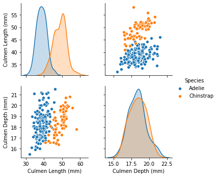
We can observe that we have quite a simple problem. When the culmen length increases, the probability that the penguin is a Chinstrap is closer to 1. However, the culmen depth is not helpful for predicting the penguin species.

For model fitting, we will separate the target from the data and we will create a training and a testing set.

from sklearn.model_selection import train_test_split

X, y = data[culmen_columns], data[target_column]
X_train, X_test, y_train, y_test = train_test_split(
    X, y, stratify=y, random_state=0,
)

To visualize the separation found by our classifier, we will define an helper function plot_decision_function. In short, this function will fit our classifier and plot the edge of the decision function, where the probability to be an Adelie or Chinstrap will be equal (p=0.5).

def plot_decision_function(X, y, clf, title="auto", ax=None):
    """Plot the boundary of the decision function of a classifier."""
    from sklearn.preprocessing import LabelEncoder

    clf.fit(X, y)

    # create a grid to evaluate all possible samples
    plot_step = 0.02
    feature_0_min, feature_0_max = (
        X.iloc[:, 0].min() - 1,
        X.iloc[:, 0].max() + 1,
    )
    feature_1_min, feature_1_max = (
        X.iloc[:, 1].min() - 1,
        X.iloc[:, 1].max() + 1,
    )
    xx, yy = np.meshgrid(
        np.arange(feature_0_min, feature_0_max, plot_step),
        np.arange(feature_1_min, feature_1_max, plot_step),
    )

    # compute the associated prediction
    Z = clf.predict(np.c_[xx.ravel(), yy.ravel()])
    Z = LabelEncoder().fit_transform(Z)
    Z = Z.reshape(xx.shape)

    # make the plot of the boundary and the data samples
    if ax is None:
        _, ax = plt.subplots()
    ax.contourf(xx, yy, Z, alpha=0.4)
    sns.scatterplot(
        data=pd.concat([X, y], axis=1),
        x=X.columns[0],
        y=X.columns[1],
        hue=y.name,
        ax=ax,
    )
    if title == "auto":
        C = clf[-1].C if hasattr(clf[-1], "C") else clf[-1].C_
        ax.set_title(f"C={C}\n with coef={clf[-1].coef_[0]}")
    else:
        ax.set_title(title)

Un-penalized logistic regression¶

The linear regression that we previously saw will predict a continuous output. When the target is a binary outcome, one can use the logistic function to model the probability. This model is known as logistic regression.

Scikit-learn provides the class LogisticRegression which implements this algorithm.

from sklearn.linear_model import LogisticRegression

logistic_regression = make_pipeline(
    StandardScaler(), LogisticRegression(penalty="none")
)
plot_decision_function(X_train, y_train, logistic_regression)

Thus, we see that our decision function is represented by a line separating the 2 classes. Since the line is oblique, it means that we used a combination of both features:

print(logistic_regression[-1].coef_)

[[15.58970002 -6.99549891]]

Indeed, both coefficients are non-null.

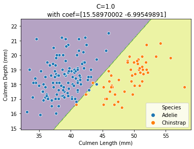
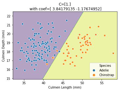
Apply some regularization when fitting the logistic model¶

The LogisticRegression model allows one to apply regularization via the parameter C. It would be equivalent to shifting from LinearRegression to Ridge. Ccontrary to Ridge, the value of the C parameter is inversely proportional to the regularization strength: a smaller C will lead to a more regularized model. We can check the effect of regularization on our model:

_, axs = plt.subplots(ncols=3, figsize=(12, 4))

for ax, C in zip(axs, [0.02, 0.1, 1]):
    logistic_regression = make_pipeline(
        StandardScaler(), LogisticRegression(C=C)
    )
    plot_decision_function(
        X_train, y_train, logistic_regression, ax=ax,
    )

A more regularized model will make the coefficients tend to 0. Since one of the features is considered less important when fitting the model (lower coefficient magnitude), only one of the feature will be used when C is small. This feature is the culmen length which is in line with our first insight when plotting the marginal feature probabilities.

Just like the RidgeCV class which automatically finds the optimal alpha, one can use LogisticRegressionCV to find the best C on the training data.

from sklearn.linear_model import LogisticRegressionCV

logistic_regression = make_pipeline(
    StandardScaler(), LogisticRegressionCV(Cs=[0.01, 0.1, 1, 10])
)
plot_decision_function(X_train, y_train, logistic_regression)

Beyond linear separation¶

As we saw in regression, the linear classification model expects the data to be linearly separable. When this assumption does not hold, the model is not expressive enough to properly fit the data. One needs to apply the same tricks as in regression: feature augmentation (potentially using expert-knowledge) or using a kernel based method.

We will provide examples where we will use a kernel support vector machine to perform classification on some toy-datasets where it is impossible to find a perfect linear separation.

from sklearn.datasets import (
    make_moons, make_classification, make_gaussian_quantiles,
)

X_moons, y_moons = make_moons(n_samples=500, noise=.13, random_state=42)
X_class, y_class = make_classification(
    n_samples=500, n_features=2, n_redundant=0, n_informative=2,
    random_state=2,
)
X_gauss, y_gauss = make_gaussian_quantiles(
    n_samples=50, n_features=2, n_classes=2, random_state=42,
)

datasets = [
    [pd.DataFrame(X_moons, columns=["Feature #0", "Feature #1"]),
     pd.Series(y_moons, name="class")],
    [pd.DataFrame(X_class, columns=["Feature #0", "Feature #1"]),
     pd.Series(y_class, name="class")],
    [pd.DataFrame(X_gauss, columns=["Feature #0", "Feature #1"]),
     pd.Series(y_gauss, name="class")],
]

from sklearn.svm import SVC

_, axs = plt.subplots(ncols=3, nrows=2, figsize=(12, 9))

linear_model = make_pipeline(StandardScaler(), SVC(kernel="linear"))
kernel_model = make_pipeline(StandardScaler(), SVC(kernel="rbf"))

for ax, (X, y) in zip(axs[0], datasets):
    plot_decision_function(X, y, linear_model, title="Linear kernel", ax=ax)
for ax, (X, y) in zip(axs[1], datasets):
    plot_decision_function(X, y, kernel_model, title="RBF kernel", ax=ax)

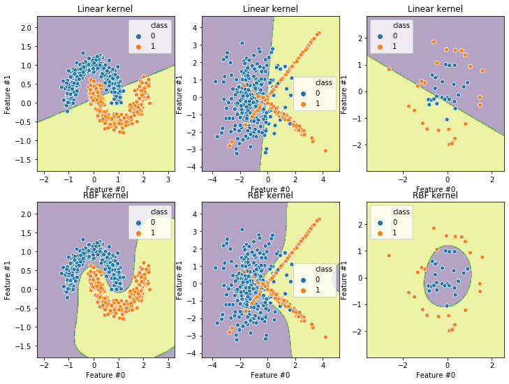
We see that the \(R^2\) score decreases on each dataset, so we can say that each dataset is “less linearly separable” than the previous one.

Scikit-learn tutorial