Comparing model performance with a simple baseline

In this notebook, we present how to compare the generalization performance of a model to a minimal baseline. In regression, we can use the DummyRegressor class to predict the mean target value observed on the training set without using the input features.

We now demonstrate how to compute the score of a regression model and then compare it to such a baseline on the California housing dataset.

Note

If you want a deeper overview regarding this dataset, you can refer to the section named “Appendix - Datasets description” at the end of this MOOC.

from sklearn.datasets import fetch_california_housing

data, target = fetch_california_housing(return_X_y=True, as_frame=True)
target *= 100  # rescale the target in k$

Across all evaluations, we will use a ShuffleSplit cross-validation splitter with 20% of the data held on the validation side of the split.

from sklearn.model_selection import ShuffleSplit

cv = ShuffleSplit(n_splits=30, test_size=0.2, random_state=0)

We start by running the cross-validation for a simple decision tree regressor which is our model of interest. Besides, we will store the testing error in a pandas series to make it easier to plot the results.

import pandas as pd
from sklearn.tree import DecisionTreeRegressor
from sklearn.model_selection import cross_validate

regressor = DecisionTreeRegressor()
cv_results_tree_regressor = cross_validate(
    regressor, data, target, cv=cv, scoring="neg_mean_absolute_error", n_jobs=2
)

errors_tree_regressor = pd.Series(
    -cv_results_tree_regressor["test_score"], name="Decision tree regressor"
)
errors_tree_regressor.describe()

count    30.000000
mean     45.663756
std       1.214956
min      43.682669
25%      44.796011
50%      45.753914
75%      46.558999
max      47.997163
Name: Decision tree regressor, dtype: float64

Then, we evaluate our baseline. This baseline is called a dummy regressor. This dummy regressor will always predict the mean target computed on the training target variable. Therefore, the dummy regressor does not use any information from the input features stored in the dataframe named data.

from sklearn.dummy import DummyRegressor

dummy = DummyRegressor(strategy="mean")
result_dummy = cross_validate(
    dummy, data, target, cv=cv, scoring="neg_mean_absolute_error", n_jobs=2
)
errors_dummy_regressor = pd.Series(
    -result_dummy["test_score"], name="Dummy regressor"
)
errors_dummy_regressor.describe()

count    30.000000
mean     91.140009
std       0.821140
min      89.757566
25%      90.543652
50%      91.034555
75%      91.979007
max      92.477244
Name: Dummy regressor, dtype: float64

We now plot the cross-validation testing errors for the mean target baseline and the actual decision tree regressor.

all_errors = pd.concat(
    [errors_tree_regressor, errors_dummy_regressor],
    axis=1,
)
all_errors

	Decision tree regressor	Dummy regressor
0	46.252221	90.713153
1	47.122262	90.539353
2	44.230612	91.941912
3	43.731460	90.213912
4	47.997163	92.015862
5	45.170314	90.542490
6	43.955949	89.757566
7	44.450599	92.477244
8	44.940107	90.947952
9	44.747979	91.991373
10	47.008742	92.023571
11	45.803452	90.556965
12	45.093547	91.539567
13	45.811914	91.185225
14	46.741463	92.298971
15	43.885867	91.084639
16	45.971291	90.984471
17	46.504399	89.981744
18	45.142408	90.547140
19	46.980128	89.820219
20	43.682669	91.768721
21	46.315907	92.305556
22	45.704375	90.503017
23	46.577199	92.147974
24	46.648009	91.386320
25	45.691297	90.815660
26	44.139437	92.216574
27	46.302171	90.107460
28	45.439936	90.620318
29	47.869812	91.165331

import matplotlib.pyplot as plt
import numpy as np

bins = np.linspace(start=0, stop=100, num=80)
all_errors.plot.hist(bins=bins, edgecolor="black")
plt.legend(bbox_to_anchor=(1.05, 0.8), loc="upper left")
plt.xlabel("Mean absolute error (k$)")
_ = plt.title("Cross-validation testing errors")

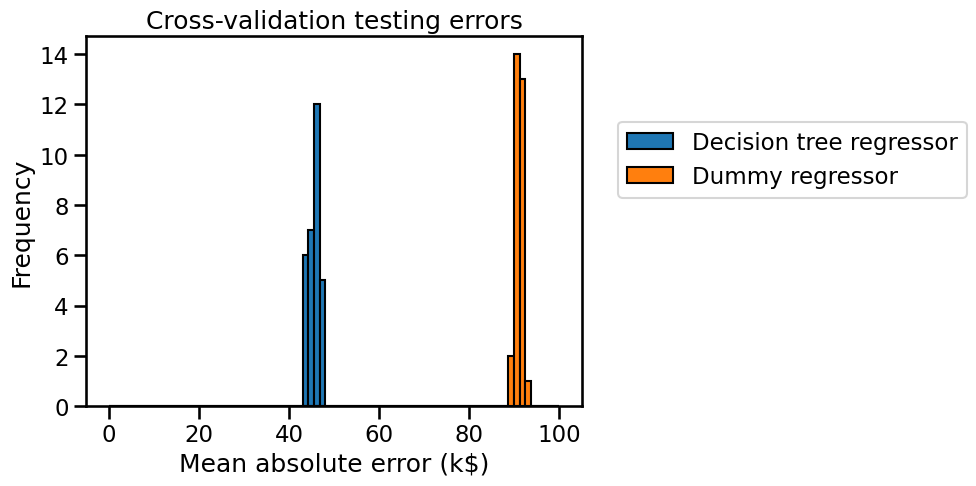
We see that the generalization performance of our decision tree is far from being perfect: the price predictions are off by more than 45,000 US dollars on average. However it is much better than the mean price baseline. So this confirms that it is possible to predict the housing price much better by using a model that takes into account the values of the input features (housing location, size, neighborhood income…). Such a model makes more informed predictions and approximately divides the error rate by a factor of 2 compared to the baseline that ignores the input features.

Note that here we used the mean price as the baseline prediction. We could have used the median instead. See the online documentation of the sklearn.dummy.DummyRegressor class for other options. For this particular example, using the mean instead of the median does not make much of a difference but this could have been the case for dataset with extreme outliers.